Guide to Long Short Term Memory (LSTM) models in Stock Prediction
How to predict daily stock prices in a more accurate way

Stock market prediction is the process to determine the future value of company stock or other financial instruments traded on an exchange. The successful forecast of a stock’s future price could yield significant profit. My motivation in this project is that a good prediction helps us make better financial decisions (buy or sell) about the future. The main objective is to identify a high price for the next day to understand the movement of stocks in the market. Hence, I worked on a stock dataset in Kaggle and will be talking about how to build a neural network model via Python.
Packages used: TensorFlow, Keras, Sklearn, Matplotlib, Seaborn and Plotly
Neural Networks have become more popular in machine learning and have applications in many areas, including image recognition and classification, speech recognition, robotics, machine translation and financial forecasting. In financial forecasting, statistical methods (Moving Average, Exponential Models, ARIMA) and machine learning models (Random Forest, Gradient Boosting, etc…) are generally used in the forecasting area. In addition to these methods, many people started using neural network models in the last 40 years. Neural networks are a set of algorithms, which are built to recognize patterns in time series data.
Introduction to Recurrent Neural Network and Long Short Term Memory
The idea behind Recurrent Neural Networks (RNNs) is to handle sequential information (connect past information to the current). RNNs are called recurrent because once the output of the network is produced, the output is copied and returned to the network as input. In a decision process, not only the current input and output are analyzed, but the previous input is also considered. In another way, they have a “memory” that retains information about what has been calculated so far. However, they are limited to looking back only a few steps in practice.

LSTMs were introduced by Hochreiter & Schmidhuber (1997), and they are explicitly designed to avoid the long-range issue that a vanilla RNN faces. They are slightly different than RNNs by using a different function to compute the hidden state. LSTM network consists of several memory blocks called cells. Two states are being passed to the next cell; the cell state and the hidden state. The LSTMs can add or remove information to the cell state via gates.
An LSTM cell has 5 vital components that allow it to utilize both long-term and short-term data: the cell state, hidden state, input gate, forget gate and output gate.
- Forget gate layer: The decision of what information is going to pass from the cell state is done by the “forget gate layer.” It gives a number between 0 and 1 for each number in the cell state by using the sigmoid function. While 1 shows “let input through”, 0 means “do not let input through”.
- Input gate layer: It manages the process of the addition of information to the cell state (decide which values to update). Firstly, it regulates what values need to be added to the cell state by using a sigmoid function. Then, it creates a vector including all possible values that can be added to the cell state by using the tanh function, which outputs values from -1 to +1. It multiplies the value of the filter (the sigmoid gate) to the created vector (the tanh function) and so it transfers this useful information to the cell state via addition operation.
- Output gate layer: In that step, the network selects useful information from the current cell state and shows as output is done via the output gate.
Dataset
The dataset from NASDAQ and NYSE includes 851,264 rows and 6 columns. The financial data comprises open, close, low and high prices of stocks and volume of stocks. Prices were fetched from Yahoo Finance and the obtained time-series data includes historical, 6 years of daily observations, from 2010–01–04 to 2016–12–30. There are 501 different company stocks in the data such as Walmart, Google, Apple, Starbucks, Amazon and Facebook.

Data Exploration and Processing
Firstly, I checked the quality of the dataset. All data types are integer in the data and it does not have any missing values/observations in the historical data. Afterward, I analyzed the distribution of the companies over sectors in the dataset. There are 11 different sectors and the companies in ‘Consumer Discretionary’, ‘Industrials’, ’IT’ and ‘Finance’ accounted for 57 % of the total companies (Figure 3).

Figure 4 demonstrates several stock prices of Google company (open, close, high and low) over 5 years starting from 2010. Stock prices almost quadrupled in the past 5 years.

In addition to that, we checked the difference between consecutive periods to understand the fluctuations. For example, when we plotted the price changes of ‘Google’ stocks over historical periods and looked at the probability density of price changes, Figure 5 shows that although there have been significant changes between 2015 and 2016, there has been normal distribution on differences.

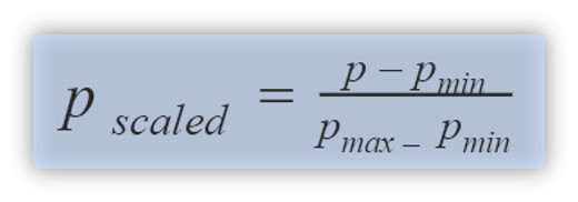
Before the modeling part, we normalized stock prices by using min-max normalization for each stock. The goal of normalization is to change the values of price columns in a dataset to a common scale without distorting differences in the range of the values. This can be applied when features have different ranges (scales of inputs are wildly different).

With normalized values, we executed the LSTM model on train and validation data and then reached forecasting values by denormalizing predictions.
Forecasting Approach
The LSTM model makes a set of predictions based on a window of consecutive samples from the historical data. We used a window of 21 when training the LSTM model, meaning that the model utilizes the previous 21 days when predicting the upcoming day’s stock price. Specifically, we are trying to predict the “high price”, and we are training the LSTM separately for each company in the dataset. Figure 7 demonstrates the fundamental idea of window size in the forecasting model.

In the forecasting model, I used 90% of historical data as train data and the remaining represents validation data.
Modeling
I designed the LSTM model by defining neuron sizes, the number of layers, optimizers and loss.
- Neuron size: 32, 64, 128
- The number of layers: 2, 4, 6
- Optimizers: SGD, Adam, AdaDelta
- Loss: MSE, MAE, RMSE
As a result of the experimental design above, the LSTM model includes 2 LSTM layers with 64 neurons and 2 layers with ReLu and linear activation functions (total of 4 layers). To regularize the neural network, I added ‘dropout’ to the LSTM layers. Probabilistically dropping out of nodes in the network is an effective method to avoid overfitting. During training, several layer outputs are randomly ignored (dropout value is 0.3).
Then, I defined the loss function by using Mean Absolute Error (MAE). I selected ‘Adam’ optimizer in the optimization part of the neural network since this resulted in much better results.

I plotted the loss over 30 epochs for the Google stock and determined that the loss doesn’t seem to improve much after 13 epochs. This was also true for other stocks that I checked, such as Amazon, Apple, Uber and Starbucks. Therefore, for computational efficiency, we decided only to run 13 epochs as shown in Figure 9.

Then, I executed the LSTM model for each stock by using the code below and saved forecasted values in the validation data.
Evaluation
To evaluate the performance of the forecasting, I computed the forecasting bias and accuracy of each stock by using formulas defined below.

The evaluation objective is to reach a low bias and high accuracy value. ‘Bias’ shows whether the forecasting model is overshooting or undershooting. Figure 11 points out the forecasting bias of several stocks. For example, the forecasting bias of AAPL stock is 0.82% which means our model is slightly overshooting.

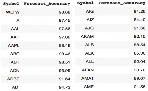
In addition to that, the ‘accuracy’ demonstrates how the forecasting model fits with actual observations. Figure 12 illustrates the forecasting accuracy of the same stocks among 501 stocks. Generally, the forecasting accuracy of LSTM models on stocks is higher than 85%.

Subsequently, I plotted the forecast accuracy of all stocks to understand how the model performs on the entire stock portfolio by looking at the histogram below. As Figure 13 shows, the forecasting accuracy of 468 stocks among 501 stocks is higher than 85% with the LSTM model. Average forecasting accuracy of all stocks is 94.4%.

I would like to illustrate how the model fits actual observations for several stocks. Figure 14 visualizes actual and forecasted values for SWK stock with 95.3 % forecast accuracy. The model can identify the general pattern on the validation data although there is still some discrepancy between actual and predicted values.

As shown in Figure 15, the model can capture all patterns and changes of DTE stock (with 97.5 % accuracy) on the validation data with smaller residual errors.

These examples indicate that LSTM can capture time-series patterns by taking advantage of both long term and short term memory, so it resulted in higher forecasting accuracy and low bias.
Takeaways
I wanted to summarize advantages and disadvantages of neural network models in forecasting. Besides, I underlined a couple of facts related to stock prediction cases.
Pros:
- The stock market can be a little bit risky but the payoff will be much higher. Therefore, stock prediction cases are one of the hot topics in the investment & banking sector.
- As this post demonstrates, the neural network model is capable of learning time series patterns by looking at historical data (exploring non-linear and complex relationships).
- Given sufficient data, you should be able to train a neural network and achieve desired results.
Cons:
- Stock markets are very volatile and stocks’ values are highly affected by external factors such as politics, unexpected events, natural calamities and fluctuations in exchange rates. For instance, as we all experienced in 2020, the world suffered from coronavirus and stock market crashed subsequently. Neural networks would have difficulty in responding to and learning from such unpredictable events.
- With the LSTM model, I observed extremely good accuracies for most stocks, specifically the ones with regular pattern. Not every stock though follows such a decodable pattern making it harder to predict.
- In order to avoid overfitting, one should pay special attention to configuring parameters of a neural network model such as number of layers, neuron sizes, activation functions, optimizers and losses.
Next Steps
I am planning to add internal and external drivers to the existing model to improve the interpretability of neural networks (industry average, competitor index, macro economics indicators) to explain existing forecasting bias and error. Furthermore, I would test whether clustering stocks based on sectors (tech, finance, energy, food services, etc…) and then developing tailored neural network enhances the performance of the prediction model.
The goal of this post was to provide a practical guide to neural networks for forecasting time series data using the LSTM approach. Please leave any comment you have and also if you would like me to explain anything further!
